import matplotlib.pyplot as pltimport matplotlib.ticker as mtickimport plotly.graph_objects as goimport numpy as npimport sympy as smfrom itertools import cycleimport pandas as pdimport statsmodels.api as statsnp.random.seed(10)
Introduction
This article is the 3rd, and final, in a 3 part series. In the 1st part, we studied basic optimization theory. Then, in pt. 2, we extended this theory to constrained optimization problems. Now, in pt. 3, we will apply the optimization theory covered, as well as econometric and economic theory, to solve a profit maximization problem.
Suppose, as a data scientist working for your company, you are tasked with estimating the optimal amount of money to allocate towards different advertising channels that will maximize the overall profit of a certain product line. Furthermore, suppose you are given constraints on these allocation decisions, such as the maximum total spend you have to allocate and/or minimum amounts that have to spent in certain channels. In this article, we are going to combine the optimization theory covered in part 1 and part 2 of this series, along with additional economic and econometric theory to tackle a theoretical profit maximization problem of this sorts — which we will flesh out in more detail in this article.
The goal of this article is to tie together what we have learned thus far and my hope is to motivate and inspire readers on how to incorporate these techniques into an applied setting. It is not meant to be a comprehensive solution to the problem covered as nuances and idiosyncrasies can, of course, complicate theoretical examples. Furthermore, many of the techniques covered have much more optimized implementations in python via packages such as pyomo, SciPy, etc. Nevertheless, I hope to provide a strong framework for constructing applied optimization problems. Let’s dive into it!
Optimization Theory - Parts 1 & 2 Recap
Brief Recap: In part 1, we covered basic optimization theory — including 1) setting up and solving a simple single variable optimization problem analytically, 2) iterative optimization schemes — namely, gradient descent & Newton’s Method, and 3) implementing Newton’s method by hand and in python for a multi-dimensional optimization problem. In part 2, we covered constrained optimization theory — including 1) incorporating equality constraints and 2) incorporating inequality constraints into our optimization problems and solving them via Newton’s Method. This article is designed to be accessible for those who are already familiar with the content covered in part 1 and part 2.
A mathematical optimization problem can be formulated abstractly as follows:
where we choose real values of the vector \(\mathbf{x}\) that minimize the objective function \(f(x)\) (or maximize \(-f(x)\)) subject to the inequality constraints \(g(x)\) and equality constraints \(h(x)\). In part 2, we discussed how to incorporate these constraints directly into our optimization problem. Notably, using Lagrange Multipliers and Logarithmic Barrier functions we can construct a new objective function \(\mathcal{O}(\mathbf{x}, \Lambda, \rho)\):
where \(\Lambda\) is the vector of Lagrange multipliers associated with each equality constraints \(h(x)\) and \(\rho\) is the barrier parameter associated with all of the inequality constraints \(g(x)\). We can then solve this new objective function iterating by choose a starting value \(\rho\) (note that large functional values of the objective function will require much larger starting values of \(\rho\) to scale the penalization), optimize the new objective function evaluated at \(\rho\) using Newton’s method iterative scheme, then update \(\rho\) by slowly decreasing it (\(\rho \rightarrow 0\)), and repeat until convergence — where Newton’s Method iterative scheme is as follows:
where \(\mathbf{H}(\mathbf{x})\) and \(\nabla f(x)\) denote the Hessian and gradient of our objective function \(\mathcal{O}(\mathbf{x}, \Lambda, \rho)\), respectively. Convergence is obtained when we reach convergence across one or more of the following criteria:
In python, utilizing SymPy, we have 4 functions. A function that obtains the gradient of our SymPy function, the Hessian of our SymPy function, solves unconstrained optimization problem via Newton’s method, and solves a constrained optimization problem via Newton’s method according to the generalization eq. (2).
To solve a constrained optimization problem, we can run the following code (Make sure starting values are in the feasible range of inequality constraints!):
Functions Defined in Part 1 & Part 2
def get_gradient( function: sm.Expr, symbols: list[sm.Symbol], x0: dict[sm.Symbol, float], # Add x0 as argument) -> np.ndarray:""" Calculate the gradient of a function at a given point. Args: function (sm.Expr): The function to calculate the gradient of. symbols (list[sm.Symbol]): The symbols representing the variables in the function. x0 (dict[sm.Symbol, float]): The point at which to calculate the gradient. Returns: numpy.ndarray: The gradient of the function at the given point. """ d1 = {} gradient = np.array([])for i in symbols: d1[i] = sm.diff(function, i, 1).evalf(subs=x0) # add evalf method gradient = np.append(gradient, d1[i])return gradient.astype(np.float64) # Change data type to floatdef get_hessian( function: sm.Expr, symbols: list[sm.Symbol], x0: dict[sm.Symbol, float],) -> np.ndarray:""" Calculate the Hessian matrix of a function at a given point. Args: function (sm.Expr): The function for which the Hessian matrix is calculated. symbols (list[sm.Symbol]): The list of symbols used in the function. x0 (dict[sm.Symbol, float]): The point at which the Hessian matrix is evaluated. Returns: numpy.ndarray: The Hessian matrix of the function at the given point. """ d2 = {} hessian = np.array([])for i in symbols:for j in symbols: d2[f"{i}{j}"] = sm.diff(function, i, j).evalf(subs=x0) hessian = np.append(hessian, d2[f"{i}{j}"]) hessian = np.array(np.array_split(hessian, len(symbols)))return hessian.astype(np.float64)def newtons_method( function: sm.Expr, symbols: list[sm.Symbol], x0: dict[sm.Symbol, float], iterations: int=100, tolerance: float=10e-5, verbose: int=1,) ->dict[sm.Symbol, float] orNone:""" Perform Newton's method to find the solution to the optimization problem. Args: function (sm.Expr): The objective function to be optimized. symbols (list[sm.Symbol]): The symbols used in the objective function. x0 (dict[sm.Symbol, float]): The initial values for the symbols. iterations (int, optional): The maximum number of iterations. Defaults to 100. tolerance (float, optional): Threshold for determining convergence. verbose (int, optional): Control verbosity of output. 0 is no output, 1 is full output. Returns: dict[sm.Symbol, float] or None: The solution to the optimization problem, or None if no solution is found. """ x_star = {} x_star[0] = np.array(list(x0.values()))if verbose !=0:print(f"Starting Values: {x_star[0]}")for i inrange(iterations): gradient = get_gradient(function, symbols, dict(zip(x0.keys(), x_star[i]))) hessian = get_hessian(function, symbols, dict(zip(x0.keys(), x_star[i]))) x_star[i +1] = x_star[i].T - np.linalg.inv(hessian) @ gradient.Tif np.linalg.norm(x_star[i +1] - x_star[i]) < tolerance: solution =dict(zip(x0.keys(), [float(x) for x in x_star[i +1]]))if verbose !=0:print(f"\nConvergence Achieved ({i+1} iterations): Solution = {solution}" )breakelse: solution =Noneif verbose !=0:print(f"Step {i+1}: {x_star[i+1]}")return solutiondef constrained_newtons_method( function: sm.Expr, symbols: list[sm.Symbol], x0: dict[sm.Symbol, float], rho_steps: int=100, discount_rate: float=0.9, newton_method_iterations: int=100, tolerance: float=10e-5,) ->dict[sm.Symbol, float] |None:""" Performs constrained Newton's method to find the optimal solution of a function subject to constraints. Args: function (sm.Expr): The function to optimize. symbols (list[sm.Symbol]): The symbols used in the function. x0 (dict[sm.Symbol, float]): The initial values for the symbols. rho_steps (int, optional): The number of steps to update rho. Defaults to 100. discount_rate (float, optional): The scalar to discount rho by at each step. Default is 0.9. newton_method_iterations (int, optional): The maximum number of iterations in Newton Method internal loop. Defaults to 100. tolerance (float, optional): Threshold for determining convergence. Returns: dict[sm.Symbol, float] or None: The optimal solution if convergence is achieved, otherwise None. """ rho =list(x0.keys())[-1] optimal_solutions = [] optimal_solutions.append(x0)for step inrange(rho_steps):if step %10==0:print("\n"+"==="*20)print(f"Step {step} w/ rho={optimal_solutions[step][rho]}")print("==="*20+"\n")print(f"Current solution: {optimal_solutions[step]}") function_eval = function.evalf(subs={rho: optimal_solutions[step][rho]}) values = optimal_solutions[step].copy()del values[rho] optimal_solution = newtons_method( function_eval, symbols[:-1], values, iterations=newton_method_iterations, tolerance=tolerance, verbose=0, ) optimal_solutions.append(optimal_solution)# Check for overall convergence current_solution = np.array( [v for k, v in optimal_solutions[step].items() if k != rho] ) previous_solution = np.array( [v for k, v in optimal_solutions[step -1].items() if k != rho] )if np.linalg.norm(current_solution - previous_solution) < tolerance: overall_solution = optimal_solutions[step]del overall_solution[rho]print(f"\n Overall Convergence Achieved ({step} steps): Solution = {overall_solution}\n" )breakelse: overall_solution =None# Update rho optimal_solutions[step +1][rho] = ( discount_rate * optimal_solutions[step][rho] )return overall_solution
Code
x, y, λ, ρ = sm.symbols("x y λ ρ")# f(x): 100*(y-x**2)**2 + (1-x)**2# h(x): x**2 - y = 2# g_1(x): x <= 0# g_2(x) y >= 3combined_objective = (100* (y - x**2) **2+ (1- x) **2+ λ * (x**2- y -2)- ρ * sm.log((-x) * (y -3)))Gamma = [x, y, λ, ρ] # Function requires last symbol to be ρ!Gamma0 = {x: -15, y: 15, λ: 0, ρ: 10}constrained_newtons_method(combined_objective, Gamma, Gamma0)
If the material above felt foreign or you need a more rigorous recap, then I recommend taking a look at part 1 and part 2 of this series which will provide a more in-depth survey of the material above. For the remainder of this article, we will first discuss basic profit maximization & econometric theory and then move into solving the theoretical example.
Applied Profit Maximization
Problem: Suppose we have a $100,000 advertising budget and all of it must be spent. We are tasked with choosing the optimal amount of this budget to allocate towards two types of advertisement channels (digital ads and television ads) that maximize the overall profit for a particular product line. Furthermore, suppose that we must allocate at a minimum of $20k to television advertising and $10k to digital advertising.
Theoretical Formulation
Let’s now mathematically formulate the profit maximization problem we seek to solve:
where \(\pi(\cdot)\) denotes the profit function, \(\delta\) denotes digital ad spend, \(\tau\) denotes television ad spend, and \((\cdot)\) is a placeholder for additional variables. Note that we are minimizing the negative of \(\pi(\cdot)\) which is equivalent to maximizing \(\pi(\cdot)\). The profit function is defined as follows:
where \(p\) denotes the price, \(q(\delta, \tau, \cdot)\) denotes the quantity demanded function, and \(\mathcal{C}(q(\cdot), \delta, \tau)\) denotes the cost function which, intuitively, is a direct function of the quantity (if we make more it will cost more to produce) and how much we spend on advertising. The cost function can also take on additional inputs, but for the sake of demonstration we will keep it as a function of quantity and advertising costs. Notice that our choices of \(\delta\) and \(\tau\) impact the profit function directly through their impact of quantity demanded and the cost function. In order to add tractability to our optimization problem, we will need to use econometric techniques to estimate our quantity function. Once we have specified our cost function and estimated the quantity function, we can then solve our optimization problem as follows:
where \(\hat{q}\) is our estimated econometric model for quantity demanded. Before we lay out the econometric specification of our quantity model, it is necessary that we discuss an important note regarding the required assumptions for this optimization problem to prove tractable. It is imperative that we obtain the causal estimates of digital and television advertising on the quantity demanded. In the economists jargon, digital and television advertising need be exogenous in the econometric model. That is, they are uncorrelated with the error in the model. Exogeneity can be achieved in two ways: 1) We have the correct structural specification of the econometric model for the impact of digital and television advertising on quantity demanded (i.e., we include all of the relevant variables that are correlated with both quantity demanded and digital & television advertising spend) or 2) We have random variation of digital & television advertising spend (this can be achieved from randomly varying spend over time to see how demand responds).
Intuitively, exogeneity is required because it is necessary to capture the causal impact of changing advertising spend — that is, what will happen, on average, if we change the values of the advertising spend. If the effect we estimate is not causal then the changes we make in advertising spend will not correspond to the true change in quantity demanded. Note the model need not make the best predictions for quantity demanded, but rather accurately capture the causal relationship.
Let’s now suppose we specify the following econometric model for quantity demanded indexed by time t:
where \(\beta\) and \(\gamma\) are the estimates of the impact of the natural log of digital ad spend, \(\delta\), and television ad spend, \(\tau\), respectively. Additionally, \(\alpha\) is our intercept, \(\phi_1\) and \(\phi_2\) are estimates of the autoregressive components of quantity demanded, \(\mathcal{S}\) denotes seasonality, \(\mathbf{X}\) is the set of all relevant covariates and lagged covariates along with the matrix of their coefficient estimates \(\Omega\), and \(\epsilon\) is the error term. Furthermore, assume that digital and television advertising satisfy the exogeneity assumption conditional on \(\mathbf{X}\), \(\mathcal{S}\), and the autoregressive components within our model. That is,
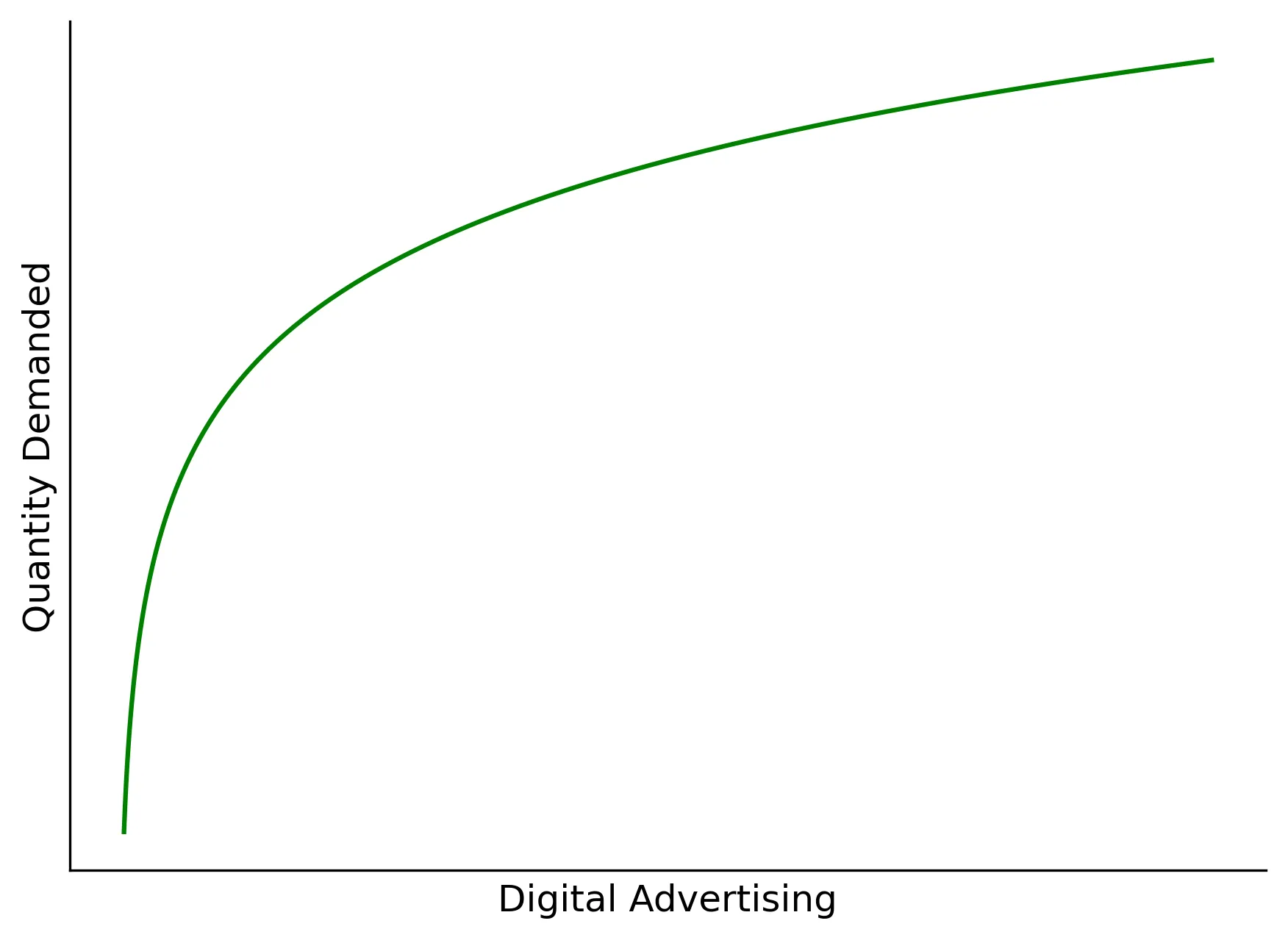
Why the natural log of digital and television ad spend you may ask? This is by no means a required nor a definitive decision in this context, but I am seeking to demonstrate how variable transformations can capture hypotheses about the relationship between our choice variables and the outcomes of interest. In our case, suppose we hypothesize that the impact on ad spend increases sharply initially, but gradually levels out (e.g., saturation effects or the law of diminishing returns). This is exactly what the logarithm transformation will allow us to model. Observe:
Here we can see that we have a cost \(\zeta\) associated with each unit produced and this cost is discounted as we produce more (think a discount for larger contracts or economies of scale). We also simply sum digital ad spend and television ad spend into our total cost.
Now that we have developed the theoretical basis for our econometric profit maximization problem, let’s simulate some data and take this to python!
Optional: Data Simulation
Note this section can be skipped without any loss of the primary content.
Let’s first simulate monthly data over 10 years for quantity demanded, where the following variables included are as follows:
Data Simulation
df = pd.DataFrame()## Digital Advertising - ln(δ)df["log_digital_advertising"] = np.log( np.random.normal(loc=50000, scale=15000, size=120).round())## Television Advertising - ln(τ)df["log_television_advertising"] = np.log( np.random.normal(loc=50000, scale=15000, size=120).round())## Matrix X of covariates# Lag Digital Advertisingdf["log_digital_advertising_lag1"] = df["log_digital_advertising"].shift(1)df["log_digital_advertising_lag2"] = df["log_digital_advertising"].shift(2)# Lag Television Advertisingdf["log_television_advertising_lag1"] = df["log_television_advertising"].shift(1)df["log_television_advertising_lag2"] = df["log_television_advertising"].shift(2)# Pricedf["price"] = np.random.normal(loc=180, scale=15, size=120).round()df["price_lag1"] = df["price"].shift(1)df["price_lag2"] = df["price"].shift(2)# Competitor Pricedf["comp_price"] = np.random.normal(loc=120, scale=15, size=120).round()df["comp_price_lag1"] = df["comp_price"].shift(1)df["comp_price_lag2"] = df["comp_price"].shift(2)# Seasonalitymonths = cycle(["Jan","Feb","Mar","Apr","May","June","July","Aug","Sep","Oct","Nov","Dec"])df["months"] = [next(months) for m inrange(len(df))]one_hot = pd.get_dummies(df["months"], dtype=int)one_hot = one_hot[["Jan","Feb","Mar","Apr","May","June","July","Aug","Sep","Oct","Nov","Dec"]]df = df.join(one_hot).drop("months", axis=1)## Constantdf["constant"] =1# Drop NaN (Two lags)df = df.dropna()
Code
df
log_digital_advertising
log_television_advertising
log_digital_advertising_lag1
log_digital_advertising_lag2
log_television_advertising_lag1
log_television_advertising_lag2
price
price_lag1
price_lag2
comp_price
...
Apr
May
June
July
Aug
Sep
Oct
Nov
Dec
constant
2
10.196866
11.135217
11.014177
11.155879
10.315365
10.631109
158.0
188.0
150.0
132.0
...
0
0
0
0
0
0
0
0
0
1
3
10.817255
11.373433
10.196866
11.014177
11.135217
10.315365
156.0
158.0
188.0
113.0
...
1
0
0
0
0
0
0
0
0
1
4
10.990702
11.166880
10.817255
10.196866
11.373433
11.135217
165.0
156.0
158.0
101.0
...
0
1
0
0
0
0
0
0
0
1
5
10.576407
10.918591
10.990702
10.817255
11.166880
11.373433
176.0
165.0
156.0
117.0
...
0
0
1
0
0
0
0
0
0
1
6
10.896424
11.087329
10.576407
10.990702
10.918591
11.166880
191.0
176.0
165.0
123.0
...
0
0
0
1
0
0
0
0
0
1
...
...
...
...
...
...
...
...
...
...
...
...
...
...
...
...
...
...
...
...
...
...
115
10.709227
10.946147
10.721239
10.569007
10.848094
10.891876
189.0
155.0
161.0
89.0
...
0
0
0
0
1
0
0
0
0
1
116
10.678560
10.730072
10.709227
10.721239
10.946147
10.848094
199.0
189.0
155.0
123.0
...
0
0
0
0
0
1
0
0
0
1
117
10.861246
10.520267
10.678560
10.709227
10.730072
10.946147
201.0
199.0
189.0
109.0
...
0
0
0
0
0
0
1
0
0
1
118
10.898516
10.568055
10.861246
10.678560
10.520267
10.730072
188.0
201.0
199.0
135.0
...
0
0
0
0
0
0
0
1
0
1
119
10.155063
11.106220
10.898516
10.861246
10.568055
10.520267
180.0
188.0
201.0
107.0
...
0
0
0
0
0
0
0
0
1
1
118 rows × 25 columns
Note that we include lag variables because it is highly plausible that today’s quantity demanded is a function of lagged values for many of the variables. We also control for seasonality effects by incorporation dummy variables for each month (this is one of many ways to incorporate seasonality into the model). We then specify the parameters associated with each variable as (note that these parameters are specified in the same order as the columns of the dataframe!):
We can then simulate our econometric specification (eq. 8) of quantity demanded by running quantity_demanded = np.array(df) @ params. However, note that we are missing the autoregressive components, thus we also want quantity demanded to follow an autoregressive process as mentioned above. That is, quantity demanded is also a function of its own lagged values. We include 2 lags here (AR(2) process) with respective coefficients \(\phi_1\) and \(\phi_2\). Note, we can simulate this with initial conditions \(q_0\) and \(q_{-1}\) via the following system:
def quantity_ar2_process(T, ϕ1, ϕ2, q0, q_1, ϵ, df, params): Φ = np.identity(T) # The T x T identity matrixfor i inrange(T):if i -1>=0: Φ[i, i -1] =-ϕ1if i -2>=0: Φ[i, i -2] =-ϕ2 B = np.array(df) @ params + ϵ B[0] = B[0] + ϕ1* q0 + ϕ2* q_1 B[1] = B[1] + ϕ2* q0return np.linalg.inv(Φ) @ B## Quantity Demand AR(2) component process# ParametersT =118# Time periods less two lagsϕ1=0.3# Lag 1 coefficient (ϕ1)ϕ2=0.05# Lag 2 coefficient (ϕ2)q_1 =250_000# Initial Condition q_-1q0 =300_000# Initial Condition q_0ϵ = np.random.normal(0, 5000, size=T) # Random Error (ϵ)quantity_demanded_ar = quantity_ar2_process(T, ϕ1, ϕ2, q0, q_1, ϵ, df, params)# Quantity_demanded target variabledf["quantity_demanded"] = quantity_demanded_ar# Additional covariates of lagged quantity demandeddf["quantity_demanded_lag1"] = df["quantity_demanded"].shift(1)df["quantity_demanded_lag2"] = df["quantity_demanded"].shift(2)
Code
df
log_digital_advertising
log_television_advertising
log_digital_advertising_lag1
log_digital_advertising_lag2
log_television_advertising_lag1
log_television_advertising_lag2
price
price_lag1
price_lag2
comp_price
...
July
Aug
Sep
Oct
Nov
Dec
constant
quantity_demanded
quantity_demanded_lag1
quantity_demanded_lag2
2
10.196866
11.135217
11.014177
11.155879
10.315365
10.631109
158.0
188.0
150.0
132.0
...
0
0
0
0
0
0
1
252645.380533
NaN
NaN
3
10.817255
11.373433
10.196866
11.014177
11.135217
10.315365
156.0
158.0
188.0
113.0
...
0
0
0
0
0
0
1
241347.807933
252645.380533
NaN
4
10.990702
11.166880
10.817255
10.196866
11.373433
11.135217
165.0
156.0
158.0
101.0
...
0
0
0
0
0
0
1
224523.403165
241347.807933
252645.380533
5
10.576407
10.918591
10.990702
10.817255
11.166880
11.373433
176.0
165.0
156.0
117.0
...
0
0
0
0
0
0
1
199677.085215
224523.403165
241347.807933
6
10.896424
11.087329
10.576407
10.990702
10.918591
11.166880
191.0
176.0
165.0
123.0
...
1
0
0
0
0
0
1
188898.838818
199677.085215
224523.403165
...
...
...
...
...
...
...
...
...
...
...
...
...
...
...
...
...
...
...
...
...
...
115
10.709227
10.946147
10.721239
10.569007
10.848094
10.891876
189.0
155.0
161.0
89.0
...
0
1
0
0
0
0
1
193482.213881
238647.180598
214751.967612
116
10.678560
10.730072
10.709227
10.721239
10.946147
10.848094
199.0
189.0
155.0
123.0
...
0
0
1
0
0
0
1
175027.266872
193482.213881
238647.180598
117
10.861246
10.520267
10.678560
10.709227
10.730072
10.946147
201.0
199.0
189.0
109.0
...
0
0
0
1
0
0
1
171063.412575
175027.266872
193482.213881
118
10.898516
10.568055
10.861246
10.678560
10.520267
10.730072
188.0
201.0
199.0
135.0
...
0
0
0
0
1
0
1
178942.616668
171063.412575
175027.266872
119
10.155063
11.106220
10.898516
10.861246
10.568055
10.520267
180.0
188.0
201.0
107.0
...
0
0
0
0
0
1
1
197501.078039
178942.616668
171063.412575
118 rows × 28 columns
Econometric Estimation & Profit Maximization
Let’s first use our framework in eq. (2) to transform our constrained optimization problem in eq. (7) to one in which we can solve utilizing our function constrained_newton_method() as done above:
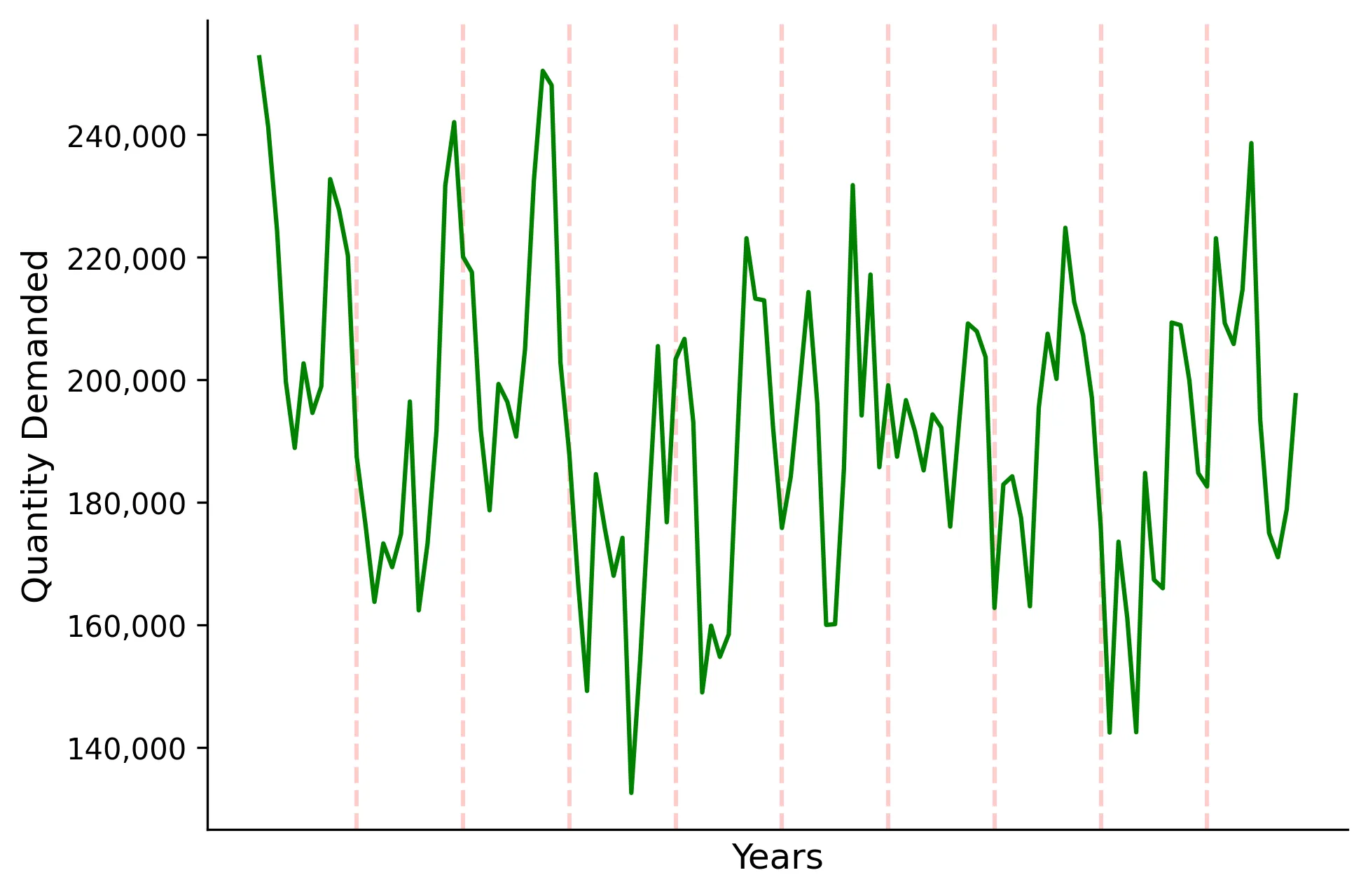
As discussed before, we need to estimate our quantity demanded, \(\hat{q}\). Let’s take a look at what our quantity demanded looks like over the 10 years simulated:
We can clearly see some seasonality occurring towards the end of the years and it appears we are dealing with a stationary process (this is all by construction). Now suppose that we have the following observed variables:
where, in eq. 8, our econometric specification, quantity_demanded is our outcome \(q\), log_digital_advertising is our \(\ln(\delta)\), log_television_advertising is our \(\ln(\tau)\), constant is our \(α\), quantity_demanded_lag1 & quantity_demanded_lag2 are our autoregressive components \(q_{t-1}\) & \(q_{t-2}\), and the remainder are our additional covariates \(\mathbf{X}\) including seasonality \(\mathcal{S}\).
Now, with this data, we seek to estimate our econometric specification in eq. 8. We can estimate this structural model using OLS. For this we will use statsmodels.
A great exercise would be to solve the linear regression using the Gradient Descent ot Newton’s method code we have constructed and compare the results to statsmodels. Hint: the objective in a linear regression is to minimize the Residual Sum of Squares. Note that the code we have written is by no means an efficient approach to solving a linear regression, but this is more oriented towards illustrating optimization theory in a model fitting (regression) context. Code for this will be provided at the end of the article!
Note that we drop the first 2 observations as these are our first two lags and we drop July as a reference month:
Code
## Fit Econometric model using OLSdf_mod = df[2:] # Drop first two lagged valuesy = df_mod["quantity_demanded"]X = df_mod.drop(["quantity_demanded", "July"], axis=1)mod = stats.OLS(y, X)results = mod.fit()print(results.summary())
Now we have our estimated econometric specification for quantity demanded! A few observations:
An increase in log digital ad spend and log television ad spend are associated with an increase in quantity demand
An increase price is associated with a decrease in quantity demand (this is expected behavior)
We see clear seasonality with increasing demand during Sep-Dec, this is consistent with our time series above
We see that the first lag of quantity demanded is predictive of the present, in favor of autoregressive process
The results above can be verified and compared with the data construction above in the data simulation section
Let’s now specify our symbolic variables for our optimization problem (\(\delta\), \(\tau\), \(\lambda\), and \(\rho\)), the values of our present variables at time \(t\), and grab the lagged values from our data. We can then obtain \(\hat{q}(\delta, \tau)\) at a point in time:
Code
# Build Symbolic Functions with all variables in functionδ, τ, λ, ρ = sm.symbols("δ τ λ ρ")## Values of current variablesprice =180comp_price =120Jan =1## Obtain Lagged Valueslog_digital_advertising_lag1 = df["log_digital_advertising"].iloc[-1]log_digital_advertising_lag2 = df["log_digital_advertising"].iloc[-2]log_television_advertising_lag1 = df["log_television_advertising"].iloc[-1]log_television_advertising_lag2 = df["log_television_advertising"].iloc[-2]price_lag1 = df["price"].iloc[-1]price_lag2 = df["price"].iloc[-2]comp_price_lag1 = df["comp_price"].iloc[-1]comp_price_lag2 = df["comp_price"].iloc[-2]quantity_demanded_lag1 = df["quantity_demanded"].iloc[-1]quantity_demanded_lag2 = df["quantity_demanded"].iloc[-2]variables = [ sm.log(δ), sm.log(τ), log_digital_advertising_lag1, log_digital_advertising_lag2, log_television_advertising_lag1, log_television_advertising_lag2, price, price_lag1, price_lag2, comp_price, comp_price_lag1, comp_price_lag2, Jan,0,0,0,0,0,0,0,0,0,0, # All Months less July1, # Constant quantity_demanded_lag1, quantity_demanded_lag2,]# Quantity Demandedquantity_demanded = (np.array([variables]) @ np.array(results.params))[0] # params from ols model
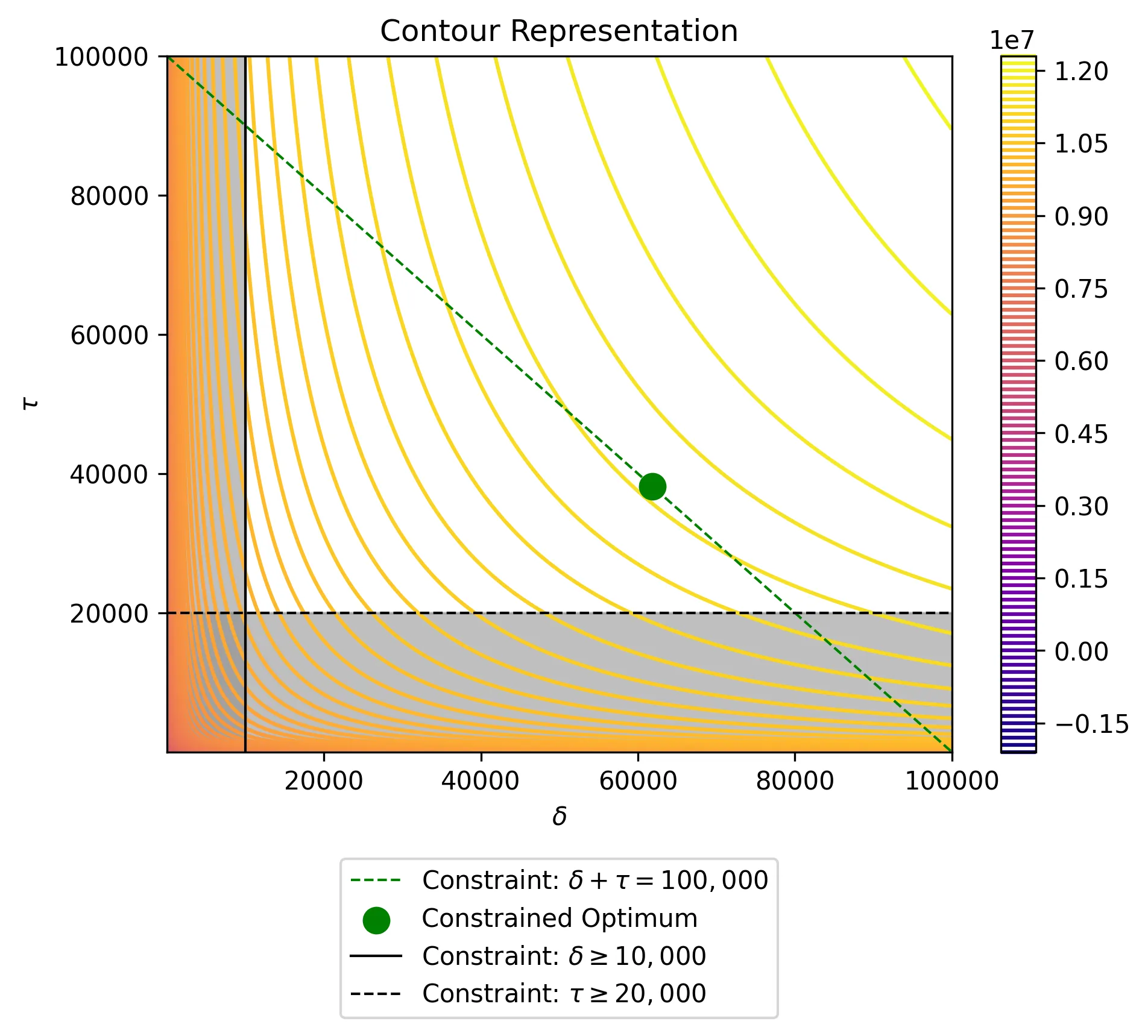
Now we can construct our revenue, cost, and put them together to construct our profit function. Here our cost to produce each unit is $140 base and is discounted by $0.0001 for each additional unit produced:
def log(x):return np.log(x)def profit_fn(δ, τ): profit_function = (-δ- τ- (-1.00712795746647* log(δ)-0.621999261508067* log(τ)+138.264406731209 )* (10071.2795746647* log(δ)+6219.99261508067* log(τ)+17355.9326879056 )+1812830.32343965* log(δ)+1119598.67071452* log(τ)+3124067.88382301 )return profit_function# Define the gridδ_grid = np.linspace(0.01, 100000, 1000)τ_grid = np.linspace(0.01, 100000, 1000)X, Y = np.meshgrid(δ_grid, τ_grid)Z = profit_fn(X, Y)# Define constraintsx_constraint = np.linspace(0, 100_000, 500)y_constraint =100_000- x_constraint# Plot contours of profit functionplt.figure(dpi=125)contour = plt.contour(X, Y, Z, levels=100, cmap="plasma")plt.colorbar(contour)plt.plot( x_constraint, y_constraint, color="green", linestyle="--", linewidth=1, label=r"Constraint: $\delta +\tau = 100,000$",)# # Mark the optimization pointsplt.scatter(61819.54,38180.46, color="green", marker="o", s=100, label="Constrained Optimum", zorder=3,)# Plot constraint linesplt.axvline(10_000, color="black", linestyle="-", linewidth=1, label=r"Constraint: $\delta \geq 10,000$",)plt.axhline(20_000, color="black", linestyle="--", linewidth=1, label=r"Constraint: $\tau \geq 20,000$",)# Shade infeasible regions in grayplt.fill_betweenx( τ_grid, 0, 10_000, color="gray", alpha=0.5) # Shade region where x > 0plt.fill_between( δ_grid, 0, 20_000, color="gray", alpha=0.5) # Shade region where y < 3# Labels and legendplt.xlabel(r"$\delta$")plt.ylabel(r"$\tau$")plt.title("Contour Representation")plt.legend(loc="lower center", bbox_to_anchor=(0.5, -0.4))plt.savefig("data/profit_function_viz_contour.webp", format="webp", dpi=300, bbox_inches='tight')
Let’s now solve our optimization problem as formulated in eq. 12 via python using the optimization theory that we have learned from part 1 and part 2 of this series. Note that the extremely high value of \(\rho\) is to account for the fact that the values of our objective function are extremely large thus we need to make sure penalization is large enough to avoid “jumping” out of constraints - we could normalize values for more stability.
Quantity: 198,064
Total Revenue: $35,651,579.11
Total Cost: $23,906,058.15
Profit: $11,745,520.95
Conclusion
The profit maximization problem in this final article was by no means meant to be an entirely comprehensive solution. In fact, we did not need to even use Newton’s Method for such a simple optimization problem! But, as optimization problems increase in complexity and dimensionality, which is quite common in the real world, these tools become increasingly relevant. The goal was to take what we have learned in part 1 and part 2 of this series and take a fun exploration into one of infinitely many applications of optimization theory.
If you have made it up to this point, thank you for taking time out of your day to read my article and I want to extend an extra thank you to those individuals that have read through all 3 parts of this series. I hope at this point you feel very comfortable with basic multi-dimensional optimization theory and extensions involving constraints on the objective function. As always, I hope you have enjoyed reading this as much as I enjoyed writing it. Please let me know what you thought of this article and the series as whole!
Bonus - Numerical and Analytical Solutions to Linear Regression
As promised above, this section will provide code for solving the linear regression problem above utilizing Newton’s method and we will compare this result to the analytical closed-form solution & statsmodels directly. This exercise will provide a very elegant connection between model fitting, optimization, & different techniques for doing this! Recall that the objective for solving the linear regression is to minimize the Residual Sum of Squares. That is, in terms of matrices,
Thus, using our Newton method function and framework, we have:
Code
def ols_newtons_method(input_df: pd.DataFrame):# Pull all variables in X and create them as SymPy symbols variablez =list(input_df.drop(["quantity_demanded", "July"], axis=1).columns) symbols = []for i in variablez: i = sm.symbols(f"{i}") symbols.append(i)# Create vectors and matrices of outcome (y), covariates (X), and parameters(β) y = np.array(input_df["quantity_demanded"]) X = np.array(input_df.drop(["quantity_demanded", "July"], axis=1)) β = np.array(symbols)# Specify objective function and starting values objective = (y - X @ β).T @ (y - X @ β) # Residual Sum of Squares β_0 =dict(zip(symbols, [0] *len(symbols)))return newtons_method(objective, symbols, β_0)β_numerical = ols_newtons_method(df_mod)
Next we will compute the analytical solution. That is, if we take the derivative of eq. A1 and set it equal to zero and solve for \(\beta\), we obtain:
I appreciate you reading my post! My posts primarily explore real-world and theoretical applications of econometric and statistical/machine learning techniques, but also whatever I am currently interested in or learning 😁. At the end of the day, I write to learn! I hope to make complex topics slightly more accessible to all.